Centering a Distribution: A Visual Guide

When you have two distributions which you suspect to have some correlation, but which feature completely disjoint values, what do you do? That was my problem last week. Specifically, I had a series of Kullback-Leibler-divergences and a series containing the percentage change of the U.S. GDP (Gross Domestic Product) over time, and I wanted to check if they correlate.

The problem is that KL-divergence is defined over the range $[0; \infty]$ and percentage changes theoretically over $[-\infty; +\infty]$ (though in reality GDP changes mostly fall somewhere between $[-10\%;+10\%]$). In other words, you can’t really compare the two distributions without any preparations.

But a colleague had a great idea: Why not center the distributions and compare them this way? Even though I roughly knew what this entailed, I wanted to double-check my intuition and thus turned to Google. A quick search for “centering a distribution” returned zero useful results. Rather, there were tons of results for tutorials that show how to “find the center of a distribution”. Disregarding the obvious fact that the “center” of a distribution is simply the mean or average, I came up short.

However, with a little bit of fiddling, I finally implemented a function myself that can center a series of values, thus rendering my two distributions comparable. The function (when implemented in numpy) involves just six short lines of code:

import numpy as np

def center_values (series: np.ndarray) -> np.ndarray:
    where_nan = np.isnan(series)
    series[where_nan] = np.nanmean(series)
    shifted_series = series - series.mean()
    centered_series = shifted_series / shifted_series.std()
    centered_series[where_nan] = np.nan
    return centered_series

Let’s quickly jump into what is happening here, first theoretically, then practically. I’ll finish off with a series of visualizations which show explicitly what is happening during centering.

Theoretical Background

When you center a distribution, what you effectively achieve is to squeeze it so that most values fall into the range $[-1;+1]$ (specifically: 95% of all values). Since this works with any distribution of any shape, this can render them comparable.

But before comparing two distributions, you first need to make sure that they are indeed comparable. Mathematically, you can center every distribution. However, when you want to compare them, you need to make sure you’re not comparing apples to oranges, lest you end up in the land of spurious correlations.

In my case, I wanted to compare two time series of change. Kullback-Leibler-divergence measures the change from one distribution to another one, i.e. I had one distribution per year, and the KL-divergence values measure how much they changed from year to year. The other distribution, GDP, should be fairly self-explanatory. I wanted to check if these two series correlate since I strongly suspected such a correlation in my case.

If you’ve cleared this path, it should be safe to compare the distributions. The next step is to actually center them. A centered distribution must have a mean of 0 ($\bar{x} = 0$) and a standard deviation of 1 ($\delta = 1$). By doing this, you render the individual values comparable between the distributions.

To center a distribution, you have to apply two operations: First shift the distribution so that its mean becomes zero and then stretch and squeeze it so that its standard deviation becomes 1. The first operation will move the distribution vertically. If you have a distribution with values greater than zero, the shift distribution will move the distribution down, and if the distribution is below zero, it will move it up. The second operation then proportionally scales every value so that they fall in the desired range, preserving the differences between the values within the distribution.

Shifting a distribution is insanely simple: You simply substract the distribution’s mean from every value. The reason why that works is simple: You can imagine the mean of a distribution as a line that goes exactly through its middle. By substracting the mean from every value, you effectively move this imaginary line until it is exactly where you want it: on the x-axis. This works even when the mean is smaller than zero: since substracting a negative value is effectively the same as adding that value, you move a distribution up if its mean is below zero.

Stretching the distribution is theoretically a little more involved. Since you want to just move all values a little bit closer to zero, the required operation here is division. You have to basically find a divisor that, when you divide every value by it, ensures that the resulting standard deviation is 1. This was actually the main reason for which I went online, because I wanted to double-check that my intuition was correct and which is where Google failed me. But my intuition proved right: The divisor we’re looking for is the standard deviation of the distribution.

At this point it makes sense to quickly reiterate the different metrics you can calculate for any distribution, and how they relate. In the following, $x_i$ describes value $i$ in the distribution, and $N$ is the number of elements in the distribution.

1. Mean: $\bar{x} = \frac{1}{N} \sum_{i=1}^{N} D_i$
2. Sum of Squares: $\text{SoS} = \sum_{i=1}^N (x_i - \bar{x})^2$
3. Variance: $\text{var}(x) = \frac{\text{SoS}}{N} = \text{SD}(x)^2$
4. Standard deviation: $SD(x) = \sqrt{var(x)}$

Basically, as you can see, you first calculate the mean, then the sum of squares (“Sum of squared deviations of the values from the distribution mean”) and the average of the sum of squares is defined as the variance. Another word for variance would also be the “spread” of the distribution. The square root of the variance is then defined as the standard deviation, or the amount by which 95% of the values spread around the mean. (A range of two times the standard deviation would include 99% of all values, and three times includes 99.9% of all values – that's also where the "significant on the 0.1%-level" speech comes from!)

For our example, dividing all values by the standard deviation will stretch or squeeze them into our target range while preserving the differences between the values themselves. A value of, e.g., $0.53$ in both centered distributions will then indicate that they’re proportionally the same (regardless of what the original, absolute value of them was in the original distributions).

Implementation

After having cleared the why, let’s move on to the how. Here, what I want to do is simply explain the function I wrote, since it contains not just the centering, but also a few safeguards that will help in the real world.

where_nan = np.isnan(series)

This line will create a list of Boolean values ([True, True, False, True]), indicating where there are NaN values in the series (NaN = Not a Number), which is a sign for missing data. You’ll encounter missing data in almost every dataset out there.

series[where_nan] = np.nanmean(series)

The second line will then replace all missing values with the mean of the non-missing values. For this I use the nanmean-function, since the regular mean-function will be unable to calculate the mean due to the missing values. The reason why this works is that we’re basically only moving along the mean of the distribution. Setting the missing values to zero (or any other arbitrary value) would distort the distribution and render the next line meaningless:

shifted_series = series - series.mean()

Here we’re performing the first transformation: Moving the distribution up or down so that the x-axis goes through the middle of it.

centered_series = shifted_series / shifted_series.std()

This line performs the second transformation and squeezes or stretches the distribution so that the standard deviation of the centered distribution becomes 1.

centered_series[where_nan] = np.nan

This last line then ensures that we’re not magically inventing data where there is none: It replaces the original missing values again with missing values. Fun fact: due to math magic™, all those values that we replaced earlier will be zero after centering. Try to think about why that is!

A Visual Guide

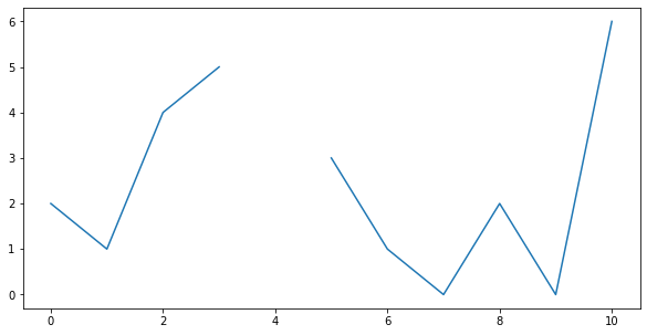
To finish off this little tutorial, here’s a visual guide of how to center a distribution. First, assume you’d have the following values: [2, 1, 4, 5, NaN, 3, 1, 0, 2, 0, 6]. When we plot it, you will see the following graph (note the gap where the missing data was):

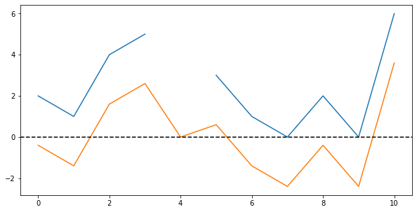
Let’s begin the centering operation by first substracting the mean from every value. If we then plot both the original and the shifted values, we see the following graph (note that the shifted distribution has no gap, and a zero in place of the missing value):

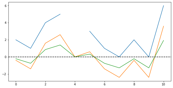
Finally, let us perform the second step in the centering operation by dividing all values by the standard deviation. Plotting all three series, we can see how the values’ range is now mostly $[-1;+1]$ except a few very large values:

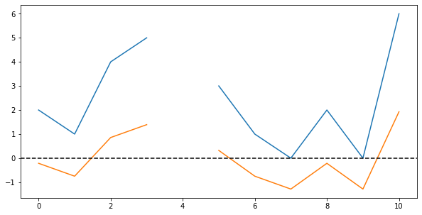
Lastly, by again replacing the former Not-a-Number-values, we can “restore” the gap in the data. Plotting both the original data and the centered values, we get this:

And that’s all you need to know about centering distributions!